Implementing ZK-focused hash schemes

In my last post, I described the ZK-oriented Ciminion AE (Dobraunig et al., 2021) scheme and implemented it using the circom2 DSL for writing zkSNARK circuits.

In this second part I present an overview of the different hashing constructions that have been proposed in the last few years, starting from MiMC (Albrecht et al., 2016) and finishing with Griffin (Grassi et al., 2022). This allows us to visit another DSL for writing SNARKs (Leo) and to explore embedded DSLs. These libraries provide APIs for constraint definition, compilation and proof generation from languages such as Go and Rust. Two examples are gnark and arkworks. Finally, I include a small list of ingredients that can be used to build a checklist when auditing circuits.

Hashing in zkSNARK circuits

In the first part of this series of articles, we dealt with encryption schemes designed for zkSNARKs applications. For instance, they can be used to prove that a certain piece of sensitive data has been encrypted using a particular key (think about cloud storage) or that a ciphertext has been correctly encrypted using a particular encryption scheme.

In general, using hashes in circuits means that a prover can convince a verifier that she knows the preimage of a value x given the hash of x (i.e. H(X)). In particular, this fact can serve to prove the knowledge of a secret, the membership of a sensitive value in a set, to obtain nullifiers and commitments, and more commonly, to implement set membership proofs in Merkle tree accumulators. In all these cases the performance of the hash scheme utilized is of utmost importance and schemes such as SHA-256 don’t provide the same performance in a circuit in comparison to a scheme based on a reduced number of multiplication and addition gates.

Structure of ZK-focused hash schemes

Typically, hashing schemes that target ZK circuits rely on the same type of linear and non-linear layers (we should note that in this article we mainly focus and describe schemes which partially or mainly optimize and measure the performance and size of their schemes using Rank-1 quadratic constraints as metric. We left schemes such as Reinforced Concrete (Grassi et al., 2021), focused on PLONK and others based on Elliptic Curve operations for another time). R1CS constraints describe a circuit via polynomials, where circuit multiplication and addition gates act over the prime Field F_p of a pairing-friendly elliptic curve. Since the proof generation complexity is generally related to the number of constraints (mainly multiplication gates, we can say additions are free), the aim of scheme designers is to reduce the number of multiplications.

In these schemes, in the linear layer, we cannot manipulate individual bits as we generally do in common block ciphers and hash functions, and matrix multiplication is used instead, via maximum distance separable (MDS) matrices for diffusion. On the other hand, non-linear layers are generally based on power maps. The smallest integer that guarantees invertibility and non-linearity is chosen. For instance

$f(x) = x^3 \mod p$

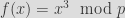
is utilized in the case of MiMC. The exponent is chosen if both

$f(x) = x^d \mod p$

and

$f(x) = x^{1/d} \mod p$

exist and are both permutations where

$gcd(p-1, a) = 1$

Most schemes are based on a round function that applies one linear layer and one non-linear layer, introducing a round constant and/or a subkey:

$R_i (x) = c + M \cdot S(x)$

where c is round constant, M is an invertible MDS matrix and S is the non-linear layer, which can be seen as an s-box. The round function is arranged in a Feistel or SPN structure and iterated. For hash constructions based on the permutations described in the next section, a sponge construction is usually instantiated.

An overview of proposed ZK-focused hash schemes

Many arithmetization-oriented schemes have been proposed in the last 7 years, targeting
multi-party computation, fully homomorphic encryption, and zero-knowledge proof applications. We provide a concise overview of constructions focused on prime fields and whose performance has been, mainly or partially measured on R1CS arithmetization. We cite block cipher designs and strategies when they have been used as inspiration to create other hash functions.

One of the first ZK-focused ciphers to be proposed was LowMC (Albrecht et al., 2016). It has received, since then, quite a lot of attention from the cryptanalysis community (see for instance here and here). Inspired by LowMC, MiMC proposes a permutation (that can use the Feistel structure), a block cipher, and a hash function. It relies on the non-linear power map x^d with x = 3. The MiMC block cipher was the starting point to improvements in encryption with the GMiMC (Grassi et al., 2019 ) construction and the HadesMiMC strategy (Grassi et al., 2019). MiMC is implemented in libraries such as circomlib and gnark.

The Poseidon hash scheme, proposed after MiMC provided two main advantages: variable-length hashes and instances dedicated for Merkle trees. It is implemented in libraries such as arkworks and circomlib. The authors followed the HadesMiMC approach and the SPN structure, together with the power map x^d, with d >= 3 (d = 5 for pairing friendly curves BLS-12-381 and BN-254). They created the Poseidon-pi permutation, based on the Hades design. It contains partial rounds (where the non-linear functions modify one part of the state) and rounds where the non-linear layer modifies the full state. The linear layer is an MDS matrix with dimensions based on the number of field elements processed by the round function.

The Rescue construction (Aly et al.,2019) it is based on a SPN network as Poseidon. However, it utilizes two non-linear layers in the same round with power maps x^a and x^1/a separated by the linear layer, which consists of a multiplication with an MDS matrix and subkey addition. Neptune is a variant of Poseidon whose non-linear layer reduces the number of multiplications. First, the authors rely on a non-linear layer that uses independent functions and second, they propose to use two different round functions: one for internal rounds and the other one for external rounds. The external round is based on the concatenation of independent s-boxes via Lai-Masey. Finally, the Griffin construction (Grassi et al., 2022) employs s-boxes inspired by Neptune and uses the so-called Horst mode of operation. It provides the best performance when used in plain for a state of field elements t >= 20 among the other candidates. And when using for membership roofs in Merkle tree accumulators it has the smallest R1CS number of constraints.

Scheme	Structure	Layers	Venue
MiMC	Feistel	Power map x^3	ASIACRYPT 2016
Poseidon	SPN	Power map x^5, MDS	USENIX Security 2021
Rescue	SPN	Power maps x^d, x^{1/d}, MDS	FSE 2020
Neptune	SPN	Independent s-boxes, MDS	ePrint 2021/1695
Griffin	SPN	Independent s-boxes, MDS	ePrint 2022/403

Summary of described zk-hash functions

In the next two sections, we implement the MiMC and Griffin permutations which allows us to describe how other DSLs for writing circuits work. Note that we only implement the permutations for demonstration purposes and that the respective sponge construction should be instantiated for real use. Also, note that to the best of our knowledge, at the time of writing this post, both Neptune and Griffin have been only published on the IACR ePrint website.

Implementing MiMC in Leo

The Leo language is utilized to create applications in the privacy-friendly blockchain Aleo. The proof related to a circuit or application written in Leo is sent as an on-chain transaction so third parties can verify the truth about a certain statement we want to prove. This structure is based on ZEXE. Leo relies on the BLS-12-337 pairing friendly curve and on the Marlin (Chiesa et al., 2019) proof system.

MiMC

In the block cipher construction, MiMC utilizes a permutation polynomial over F_q as round, consisting in the addition of the key, a round constant, and the application of a power map function:

$F_i(x) = F(x \oplus k \oplus c_i)$

And iterating over the round function F:

$E_k(x) = (F_{r-1} \circ F_{r-2} \circ$ … $\circ F_{o})(x) \oplus k$

Using the same permutation in a Feistel network, we can process two field elements if we multiply the numbers of rounds by 2. In this case, the round function is:

$x_L || x_R := x_R \oplus (x_L \oplus k \oplus c_i)^3 || xL$

Finally, the MIMC^P permutation is created by setting k = 0 and the hash function by instantiating a sponge construction with the permutation.

Power maps in the BLS-12-337 curve

Leo uses the scalar field of the BLS-12-377 curve with r = 8444461749428370424248824938781546531375899335154063827935233455917409239041.

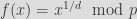
In our case, we choose a parameter d = 11. According to Section 5.1 of the MiMC paper we need that the cubing in the round function creates a permutation so gcd(3, p-1) = 1, which is not possible in the case of the scalar field of the BLS-12-377 curve. For d = 5 and d = 7 we have the same problem. We estimate the number of required rounds with the number of rounds with 2 * (log p / log d) for the power map f(x) = x^d and the permutation that uses the Feistel structure.

Implementing the MiMC^P permutation in Leo

The Leo development environment can be installed from its repository. It only requires a Rust language installation. Via the leo command-line tool, we can build, test, generate and verify proofs for a given circuit or application.

For d = 11, we require 2 * (log p / log 11) = 145 rounds. We hardcode the round constants and implement the Feistel version that can be used in the block cipher with parameter k and in the hash function with k = 0 and by instantiating a sponge construction. We start with the design of the of the non-linear layer, that comprises the addition of a round constant and the power map with d = 11:

function non_linear(state: field, constant: field) -> field {    
    let c: field = state + constant;    

    let c2: field = c*c;    
    let c4: field = c2*c2;    
    let c8: field = c4*c4;    
    let c11: field = c8*c2*c;    

    return c11;    
}

In Leo, we can create functions using the field data type, that is, an element from the curve scalar field. We add the round constant and perform the power map. The syntax is more similar to Rust than to JS. The application of one round function consists on updating the state, composed of two field elements with the addition of the result of the application of the non-linear layer:

function round(state: [field; 2], constant:field) -> [field; 2] {
    state[1] += non_linear(state[0], constant);                                                
    return state;
}

Finally, we can precompute the round constants separately and we can create the permutation:

function permutation(state: [field; 2]) -> [field; 2] {

    const N_ROUNDS:u32 = 147;

    let RC: [field; 147] = [
        3865702934124093755943890899496595264675194361091768380145853932420267718340,    
1007157542023399026163733618843871954165432315393358131261818260851607860762,    
4405765946538921025695035439523237362153599324827654321243952925829102897068,    
3664456287923997818199382200327273463939055455139573605615804006507349414661,  
[...]

    let tmp: field = 0field;

    for i in 0..N_ROUNDS - 1{                                                            
    state = round(state, RC[i]);                                                     
          tmp = state[0];                                                                  
          state[0] = state[1];                                                             
          state[1] = tmp;                                                                  
       }                                                                                    

      state = round(state, RC[N_ROUNDS - 1]);                                              

      return state;                                                                        

}

Leo allows us to create tests on the same file to test our functions, for instance, for the non-linear layer we can do:

@test
function sbox_test() {
    let constant: field = 5943928848779486925441395077146413864173255127001087220085381147547751487102 ; 
    let state: field = 5324319209727394843353330183529117967230803372202482264714325483223508628524 ;
    let check: field = 4817246075678656562069386914259487599241369120264717506466034175518663577036  ;
    let result = sbox(state, constant);

    console.assert(check == result);
}

and the round function:

@test
function round_test() {
    let state_in: [field; 2] = [
    ┆   205590015168576069906775328287417415487799853627397567932093125904979123828,
    ┆   6314658282813217945138278251984680094319698463151078319831502705046804707990 
    ];

    let constant: field = 7687545491407243578138660792989370259027838962927279562322213575702987063508;


    let result_0: field = 205590015168576069906775328287417415487799853627397567932093125904979123828;
    let result_1: field = 4768980667092361968239023698012060630723900845915064763583717922931253545522;

    let result = round(state_in, constant);

    console.assert(result_0 == result[0]);
    console.assert(result_1 == result[1]);
}

We can build the circuit and obtain the number of constraints with leo build:

$ leo build                             
     Build Starting...
     Build Compiling main program... 
     Build Number of constraints - 735
     Build Complete
      Done Finished in 23 milliseconds

as well as create proving and verification keys and a proof that can be verify correctly via leo run:

     Build Starting...
     Build Compiling main program...
     Build Number of constraints - 735
     Build Complete
      Done Finished in 38 milliseconds 

     Setup Starting...
     Setup Saving proving key 
     Setup Complete
     Setup Saving verification key 
     Setup Complete
      Done Finished in 79 milliseconds 

   Proving Starting...
   Proving Saving proof... 
      Done Finished in 54 milliseconds 

 Verifying Starting...
 Verifying Proof is valid
      Done Finished in 2 milliseconds

Implementing the Griffin permutation in gnark

So far we have used the circom2 and Leo DSLs. However, there exist other options to describe zkSNARKs circuits using embedded DSLs such as bellman, gnark and arkworks-rs. In this section, we’ll implement the Griffin permutation in gnark using the BLS-12-381 curve. These libraries create an interface between pure R1CS constraints and the operations performed in the circuit e.g. modular multiplications and additions via an API.

Introduction to gnark

We can use the gnark playground or install gnark in our project via go get. In circom2 all the signals are private by default. In gnark, signals are defined via the Circuit struct. For instance, declaring 3 (input) private signals (X₀-X₂) and 3 (output) public signals (Y₀-Y₂) is done via:

type Circuit struct {    
    X0 frontend.Variable `gnark:"x"`    
    X1 frontend.Variable `gnark:"x"`    
    X2 frontend.Variable `gnark:"x"`    

    Y0 frontend.Variable `gnark:",public"`    
    Y1 frontend.Variable `gnark:",public"`    
    Y2 frontend.Variable `gnark:",public"`    
}

Once we have defined a circuit using the arithmetic operations of the gnark front end api e.g. via api.Mul(x, x), we can obtain the R1CS representation of our circuit, for a particular curve supported by the library via:

    var myCircuit Circuit    

    // generate R1CS    
    r1cs, err := frontend.Compile(ecc.BLS12_381, r1cs.NewBuilder, &myCircuit)

after choosing a proving system (e.g. Groth16), we can perform the setup, generate the witness and the proof for verification:

    pk, vk, err := groth16.Setup(r1cs)
    witness, err := frontend.NewWitness(&myCircuit, ecc.BLS12_381)
    publicWitness, err := witness.Public()
    proof, err := groth16.Prove(r1cs, pk, witness)
    err = groth16.Verify(proof, vk, publicWitness)

but before creating the circuit for the Griffin permutation, we need to explain its structure.

The Griffin permutation non-linear layer

Grifffin improves the performance of SPN-based schemes by using the so-called Horst mode of operation and the Rescue approach. The Feistel scheme

$(x, y) := (y + F(x), x)$

is replaced by

$(x, y) := (y \cdot G(x), x)$

Griffin utilizes three non-linear functions:

$x^d$ , $x^{1/d}$ , and $(x, y) := (y \cdot G(x), x)$

where g is a quadratic function.

In our example, we chose the parameters t = 3, R = 12, d = 5, based on the BLS-12-381 field. We apply the permutation to 3 field elements. Note that we are implementing only the Griffin permutation and that we need to instantiate a sponge in order to obtain the associated hashing function. The transformation applied to the three input field elements is the following:

$y_0 = x_0^{1/d}$ , $y_1 = x_1^{d}$ , and $y_2 = x_2 \cdot ((L_i(y_0, y_1, 0))^2 + \alpha \cdot L_i ( y_0, y_1, 0) + \beta)$

The parameters alpha and beta are chosen to be distinct values where a^2 - 4*beta is a quadratic non-residue modulo p. L_i is a linear transformation:

$L_i(z_0, z_1, z_2) = \gamma_i \cdot z_0 + z_1 + z_2$

For t = 3 we obtain the following non-linear layer implementation:

func non_linear(api frontend.API, x0 frontend.Variable, x1 frontend.Variable, x2 frontend.Variable) (frontend.Variable, frontend.Variable, frontend.Variable) {

    alpha, _ := new(big.Int).SetString("20950244155795017333954742965657628047481163604901233004908207073969011285354", 10)            
    beta, _ := new(big.Int).SetString("3710185818436319233594998810848289882480745979515096857371562288200759554874", 10)

    y0 := add_chain_exp_d_inv(api, x0)        
    y1 := exp_d(api, x1)    

    // l for t = 3    
    l := api.Add(y0, y1)    
    lq := api.Mul(l, l)    
    l = api.Mul(l, alpha)    
    l = api.Add(l, lq)     
    l = api.Add(l, beta)    
    y2 := api.Mul(x2, l)     

    return y0, y1, y2    

}

The power map 1/d

At the time of writing this post, gnark does not provide a gadget for native modular exponentiation (see for instance https://github.com/ConsenSys/gnark/issues/309). We need to implement the exponentation of 1/d, that is the modular inverse of 5 mod (p -1), used on the second field element of the input in the permutation, which corresponds to z = x^0x2e5f0fbadd72321ce14a56699d73f002217f0e679998f19933333332cccccccd. Since the gnark API provides the modular multiplication operation, one alternative could be to implement a variant of the square-and-multiply approach, which would yield a number of constraints based on the number of multiplication operations (more precisely, 254 doublings and 130 multiplications = 384 multiplication gates). On other other hand, since we are dealing with a fixed exponent operation, we can implement the power map using a short addition chain. In this case, we have used addchain to generate an addition chain for 1/d based on 305 multiplications and created a template for gnark.

The Griffin permutation linear layer

The linear layer of Griffin for t = 3 is based on the circulant matrix cir(2, 1, 1), which results in adding the sum of the 3 input field elements to each of the elements of the state, that is, via the matrix:

$\begin{bmatrix} 2 & 1 & 1\\ 1 & 2 & 1\\ 1 & 1 & 2 \end{bmatrix}$

which can be performed in gnark via:

func mds_t_3_no_rc(api frontend.API, x0 frontend.Variable, x1 frontend.Variable, x2 frontend.Variable) (frontend.Variable, frontend.Variable, frontend.Variable) {

/* for t = 3, M = circ(2,1,1)    
┆  for state input (a, b, c) output is =    

┆  | 2a + b  + c  |    
┆  | a  + 2b + c  |    
┆  | a  + b  + 2c |    
*/    

sum := api.Add(x0, x1, x2)
return api.Add(sum, x0), api.Add(sum, x1), api.Add(sum, x2)

}

The permutation

Finally, we can hardcode all the round constants and perform the 12 rounds:

    rc10_0, _ := new(big.Int).SetString("0886bf20a448bd83746fe5e21995cf73911701f7ee2761575d47c44b3827dde5", 16)
    rc10_1, _ := new(big.Int).SetString("70e9886f1de2e576b86c893ddf531b467cd42ea6eb6e4273034053284ff7cb02", 16)
    rc10_2, _ := new(big.Int).SetString("4f1b3f6a9f91cfc548389964eefe28a3a9572224c5541962011b540f60b509d8", 16)

    s0, s1, s2 := mds_t_3_no_rc(api, circuit.X0, circuit.X1, circuit.X2)

    // round 1
    y0, y1, y2 := non_linear(api, s0, s1, s2)
    y0, y1, y2 = mds_t_3_rc(api, y0, y1, y2, rc0_0, rc0_1, rc0_2)

    // round 2
    y0, y1, y2 = non_linear(api, y0, y1, y2)
    y0, y1, y2 = mds_t_3_rc(api, y0, y1, y2, rc1_0, rc1_1, rc1_2)

    // round 3
    y0, y1, y2 = non_linear(api, y0, y1, y2)
    y0, y1, y2 = mds_t_3_rc(api, y0, y1, y2, rc2_0, rc2_1, rc2_2)

    // round 4
    y0, y1, y2 = non_linear(api, y0, y1, y2)
    y0, y1, y2 = mds_t_3_rc(api, y0, y1, y2, rc3_0, rc3_1, rc3_2)

[...]

Ingredients for a checklist when auditing circuits

Based on the first part of this post and this one, I have prepared a list of checks that could be used for validating implementations of zk-oriented schemes. Some of them are based on the DSL it self , others are based on the very nature of the zkSNARKs circuits themselves and finally, other mistakes can appear based on the lack of input validation of the upper layers in so-called zk-distributed applications.

Overflows not validated in upper layers

Every arithmetic operation within a circuit is performed mod q, where F_q is the field of the pairing-friendly curve utilized. That means, that if it is possible to satisfy a circuit with inputs x₀, x₁, it is also possible to satisfy the same circuit with inputs (x₀ + n*q, x₁ + n*q). Even if this fact seems trivial, an application that uses a zkSNARK circuit with authorization purposes that don’t take this fact into account can believe that is accepting different valid inputs where at the same type they correspond to the same input. This fact is directly related to the next point, “collisions” in hash functions.

“Collisions” in hash functions when input size is not validated

The same overflow example presented in the point above can be utilized for creating “collisions” in hash functions if the input is not validated in a zk-app. We can show this fact using the gnark playground. It contains an example using MiMC for proving the knowledge of a secret 0xdeadf00d with digest 5198853307513511565221857855889129613353124614036601136339058862251852610180.

// Welcome to the gnark playground!
package main

import (
	"github.com/consensys/gnark/frontend"
	"github.com/consensys/gnark/std/hash/mimc"
)

// gnark is a zk-SNARK library written in Go. Circuits are regular structs.
// The inputs must be of type frontend.Variable and make up the witness.
// The witness has a
//       * secret part --> known to the prover only
//       * public part --> known to the prover and the verifier
type Circuit struct {
	Secret frontend.Variable // pre-image of the hash secret known to the prover only
	Hash   frontend.Variable `gnark:",public"` // hash of the secret known to all
}

// Define declares the circuit logic. The compiler then produces a list of constraints
// which must be satisfied (valid witness) in order to create a valid zk-SNARK
// This circuit proves knowledge of a pre-image such that hash(secret) == hash
func (circuit *Circuit) Define(api frontend.API) error {
	// hash function
	mimc, _ := mimc.NewMiMC(api)

	// hash the secret
	mimc.Write(circuit.Secret)

	// ensure hashes match
	api.AssertIsEqual(circuit.Hash, mimc.Sum())

	return nil
}
-- witness.json --
{
    "Secret": "0xdeadf00d",
    "Hash": "5198853307513511565221857855889129613353124614036601136339058862251852610180"
}

However, if the input size is not validated in the application that uses the circuit, we can create other valid inputs, for instance 5198853307513511565221857855889129613353124614036601136339058862251852610180 + q*4 = 180304796282227713343193103817947330321740039817364875885924692354858320575116 that also satisfies the circuit. One way of avoiding this type of problems can be by enforcing input validation in the upper layer that uses the circuit. Moreover, DSLs such as circom2 allows inputs made of bits which can be used for accepting an input specific length.

Utilization of dangerous operators

Some languages include operators that can be problematic when used incorrectly. In a DSL we could expect that every assign operation including an arithmetic operator creates a constraint. This is the case when using the <== operator in circom2. However, it can be possible to assign a value including an arithmetic operation with the operator <--. In that case, a constraint is not created, which can be exploited for creating proofs with invalid inputs that pass as valid.

Finding errors in unconstrained R1CS circuits can be automated using tools such as Franklyn Wang‘s Ecne project, a tool which I contributed to during the 0xPARC 2nd learning group.

Incorrect parameters in zk-oriented schemes

Many encryption and hash schemes designed for zero-knowledge applications require round constants generated with specific properties as well as parameters (such as alpha and beta in Griffin). These parameters are usually hardcoded to reduce the number of constraints in a circuit. Another example is choosing a valid value d in the power maps according to the pairing-friendly elliptic curve utilized.

The code written for this post is available at https://github.com/kudelskisecurity/zkhash_post.

Acknowledgements

Roman Walch, Franklyn Wang (Ecne Project), 0xPARC community.

Last update: 14th July 2022

Enter your comment here...

Fill in your details below or click an icon to log in:

Email (required) (Address never made public)

Name (required)

Website

You are commenting using your WordPress.com account. ( Log Out / Change )

You are commenting using your Facebook account. ( Log Out / Change )

Cancel

Connecting to %s