


Note that this article is a hands-on, applied, comparison and does not try to explain all the details of differential privacy. For more background information on differential privacy, have a look at the references at the end of this blog post.
The promise of differential privacy (more precisely, ε-differential privacy) is to provide a measurable way to balance privacy and data accuracy when publicly releasing aggregate data on private datasets.
Imagine you have a slider that, when set to the very left end preserves total privacy of individuals in the dataset but, as a trade-off, adds a large amount of noise to the data, making aggregate stats inaccurate. That same slider, if set to the very right end, gives perfect accuracy to the aggregate stats, but at the cost of revealing private information about individuals in the dataset. The whole point here is that this very slider can be set to any point in between to suit a particular use case.
How data is transformed
ε-differential privacy lets you balance the privacy and accuracy level with a positive value named ε (epsilon). If ε is small, then more privacy is preserved but data accuracy gets worse. If ε is large, privacy will be worse but data accuracy will be preserved. Note that ε goes from 0 to infinity.
Differential privacy libraries implement various techniques that take an epsilon parameter as input and adds random noise to values in the original dataset, proportionally to the given ε parameter. Thus, the smaller the epsilon value, the more noise will be added to the values.
Some libraries will take more parameters than just ε and may allow for control over how the random noise is added to the values in the original dataset, such as the probability distribution from which random numbers should be drawn from (Laplace, Normal, etc.).
Some of those libraries also implement the concept of privacy budget, where each call to a function in the library will use up a user-defined amount of the originally allocated privacy budget. The theory behind this is that every time new information is released, the probability that an attacker retrieves information about an individual in the dataset increases. Once the privacy budget is all used up, the library may raise an error instead of returning a value.
Comparison of DP libraries
We will look at some differences between three existing differential privacy libraries and the effect on a given dataset when applying the same differentially private techniques using the following libraries:
We will have a look at how the dataset size affects accuracy and how the desired privacy level (epsilon) affects data accuracy. For each case, we will compare the results obtained using the various differential privacy libraries.
Test dataset
We randomly generate a dataset containing a single column being the weight, in kilograms, of an individual. We will consider that the weight of a person is sensible information that should be kept private. Each weight is a double value.
The weights were randomly generated according to a normal distribution where the average weight in the dataset is 70 kilograms and the standard deviation is 30.
For the needs of our research, we will make the dataset size an input parameter so that we can generate datasets a various sizes.
Here is the code that was used to simply generate the weights dataset:
import random

def generate_weight_dataset(dataset_size):
    outpath = f"weights_{dataset_size}.csv"
    mu = 70  # mean
    sigma = 30  # standard deviation
    with open(outpath, "w+") as fout:
        for i in range(dataset_size):
            random_weight = random.normalvariate(mu, sigma)  # normal distribution
            random_weight = abs(random_weight)  # make sure weights are positive
            random_weight = round(random_weight, 1)  # round to 1 decimal digit
            line = f"{random_weight}"
            print(line, file=fout)
For example, with dataset size 10600, the generated data would look like this:

The actual mean of the dataset should be roughly 70 because we used a normal distribution with mean=70. That is, however, not its exact value because weights are randomly drawn, and in addition to that, we take the absolute value of weights so that people do not have negative weights and final values are rounded to one decimal digit. In fact, the actual mean weight was 70.34812570579449, and the standard deviation was 29.488380395675765 in this example.
Note, however, that the only purpose of doing this is to have a real-life looking dataset, and the distribution of the values in the dataset will not affect the measures we are about to discuss.
Library usage
Before we start, let us see how the libraries will be used. We will always compare libraries with the same parameters. For example, the same epsilon value will be provided as input. The operation that we will use for measuring is the mean value of our dataset. These libraries implement operations such as the mean, variance, sum, etc. with underlying mechanisms that add random noise to values. One common mechanism is the use of Laplace noise. The choice of the mean operation here is arbitrary and allows to cover testing of all operations that use the same underlying mechanism.
With IBM’s library (Python), we compute the DP mean in the following way:
import diffprivlib.tools.utils

def dp_mean(weights, epsilon, upper):
    dp_mean = diffprivlib.tools.utils.mean(weights, epsilon=epsilon, range=upper)
    return dp_mean

upper = max(weights)
epsilon = 1.0
dpm = dp_mean(weights, epsilon, upper)
With Google’s library (C++), the process for computing the DP mean that was used is:
double dp_mean(std::list<double> weights, double epsilon, double lower, double upper) {
    std::unique_ptr<differential_privacy::BoundedMean<double>> mean_algorithm =
    differential_privacy::BoundedMean<double>::Builder()
    .SetEpsilon(epsilon)
    .SetLower(0.0)
    .SetUpper(upper)
    .Build()
    .ValueOrDie();

    for (auto weight : weights) {
        mean_algorithm->AddEntry(weight);
    }
    double privacy_budget = 1.0;
    auto output = mean_algorithm->PartialResult(privacy_budget).ValueOrDie();
    return differential_privacy::GetValue<double>(output);
}
Note that we use the full privacy budget of 1.0 every time when using Google’s library, since the IBM library does not take that parameter as input.
With diffpriv (R), the DP mean is computed this way:
library(diffpriv)

dp_mean <- function(xs, epsilon) {
  ## a target function we'd like to run on private data X, releasing the result
  target <- function(X) mean(X)

  ## target seeks to release a numeric, so we'll use the Laplace mechanism---a
  ## standard generic mechanism for privatizing numeric responses
  n <- length(xs)
  mech <- DPMechLaplace(target = target, sensitivity = 1/n, dims = 1)

  r <- releaseResponse(mech, privacyParams = DPParamsEps(epsilon = epsilon), X = xs)
  r$response
}
How privacy affects data accuracy
Accuracy of the mean produced by differential privacy libraries can be measured by simply computing the difference between the DP mean and the actual mean.
Let us see what happens to the accuracy of the mean weight when the value of epsilon changes. Since random noise is added, we will do 100 runs and compute the mean squared error (MSE) to verify that the library is not producing biased values.
The output should show that the error (the difference between the actual mean and the DP mean) is inversely proportional to epsilon. If epsilon is large, the error should be small, and the other way around. Values for epsilon were tested ranging from e^-10 and e^10 (notice the logarithmic scale).
For this test, an arbitrary fixed dataset size of 10’600 rows was used.
Mean squared error

We can see that indeed, the error gets smaller if epsilon gets larger. One interesting observation here is that the Google library appears to be bounded in terms of mean squared error, as the value of epsilon gets very small, whereas this is not the case for IBM’s library and neither for diffpriv.
The reason for this lies in this excerpt from the source code of Google’s library:
In numerical-mechanisms.h:
  // Adds differentially private noise to a provided value. The privacy_budget
  // is multiplied with epsilon for this particular result. Privacy budget
  // should be in (0, 1], and is a way to divide an epsilon between multiple
  // values. For instance, if a user wanted to add noise to two different values
  // with a given epsilon then they could add noise to each value with a privacy
  // budget of 0.5 (or 0.4 and 0.6, etc).
  virtual double AddNoise(double result, double privacy_budget) {
    if (privacy_budget <= 0) {
      privacy_budget = std::numeric_limits<double>::min();
    }
    // Implements the snapping mechanism defined by
    // Mironov (2012, "On Significance of the Least Significant Bits For
    // Differential Privacy").
    double noise = distro_->Sample(1.0 / privacy_budget);
    double noised_result =
        Clamp<double>(LowerBound<double>(), UpperBound<double>(), result) +
        noise;
    double nearest_power = GetNextPowerOfTwo(diversity_ / privacy_budget);
    double remainder =
        (nearest_power == 0.0) ? 0.0 : fmod(noised_result, nearest_power);
    double rounded_result = noised_result - remainder;
    return ClampDouble<double>(LowerBound<double>(), UpperBound<double>(),
                               rounded_result);
  }
In bounded-mean.h:
    // Normal case: we actually have data.
    double normalized_sum = sum_mechanism_->AddNoise(
        sum - raw_count_ * midpoint_, remaining_budget);
    double average = normalized_sum / noised_count + midpoint_;
    AddToOutput<double>(&output, Clamp<double>(lower_, upper_, average));
    return output;
Indeed, as epsilon gets very small (roughly 0.013 or less), the diversity (which is simply 1/epsilon) will become extremely large and the added noise will be zero, thus the library will return a DP mean equal to the midpoint of the bounds used for the mean. This explains the start of the red line on the chart above.
diffpriv appears to have a smaller MSE, and therefore better accuracy, overall, compared to the other two libraries, when using the same value for epsilon. To guarantee the same privacy level with diffpriv, a smaller epsilon value than the one used with the two other libraries should be used.
Standard deviation
The standard deviation of the error on 100 runs looks like:

We can see that Google’s library is pretty consistent for small epsilon values and then quickly matches IBM’s library. Overall, diffpriv has a smaller standard deviation than the other two libraries.
How dataset size affects data accuracy
Next, let us see how the dataset size affects the accuracy of the DP mean weight.
One of the risks of having a small dataset is that single individuals make large contributions to an aggregate value, such as the mean. Therefore, if our dataset contains only one individual, a perfectly accurate mean will tell the exact weight of that individual. Let us see what libraries do to avoid revealing individual information when the dataset size changes.
For this test, an arbitrary fixed value for epsilon of 1.0 was used.
Mean squared error

We can see that, as the dataset size gets smaller, the mean squared error becomes larger, and the other way around. This appears to be the expected result. If there are few individuals, we want to add extra noise to avoid revealing private data. The downside is that, for small datasets, the aggregate values may become completely irrelevant due to their inaccuracy.
As for diffpriv, the MSE varies a lot more when the dataset size changes, however, we can still see a pattern where, just like the other two libraries, the MSE becomes smaller when the dataset becomes larger. But that is only true up to a dataset size of about 30’000. From there, it appears that the MSE stays about the same, even if the dataset becomes larger. Also, notice that when the dataset size is 17912, the MSE is abnormally small.
Standard deviation
Another question we may ask ourselves is how the amount of added noise changes between each of the 100 test runs for a given dataset size. To answer this, let us plot the standard deviation of the error for 100 runs for each dataset size.
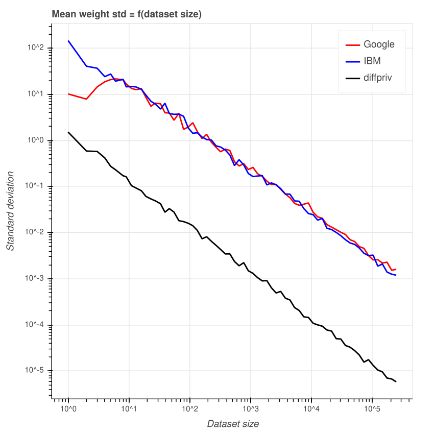
We can see that the error varies more for small datasets. However, Google’s library appears to have a peak when the dataset size is 6. Smaller datasets have less variance and larger datasets as well. This is not the case for IBM’s library where the line seems to follow a linear pattern.
Again, diffpriv appears to have a smaller standard deviation overall.
Conclusions
We have seen that the measures performed with the three differential privacy libraries happen to match the initial intuition. However, the different implementations produce different results, especially in some corner cases, such as for very small epsilon values with Google’s library. In practice, this shouldn’t be a problem since the user would not use bounds that are equal to the min and max value of the dataset and such a small epsilon value would rarely be used. However, the library may print a warning in such a case.
diffpriv appears to behave noticeably differently than the other two libraries so we advise users to be careful of the epsilon value used.
References
- Differential Privacy (Wikipedia)
- The Algorithmic Foundations of Differential Privacy
- Evaluating Laplace Noise Addition to Satisfy Differential Privacy Numeric Data
- Almost differential privacy
- Differential privacy: An illustrated primer
- Differential Privacy: A Survey of Results
- On Significance of the Least Significant Bits For Differential Privacy
