Defeating Quantum Algorithms with Hash Functions

In this post I’ll explain why quantum computers are useless to find hash function collisions, and how we can leverage this powerlessness to build post-quantum signature schemes. I’ll then describe a quantum computing model that you can try at home, and  one where hash function collisions are easy to find.

Let me start with a few background points:

• Quantum algorithms exist to efficiently solve the factoring problem (get p and q from n=p×q) and the discrete logarithm problem (get e from x=g^e mod p) With a classical computer these problems are hard, and that’s the reason why crypto schemes such as RSA or Diffie-Hellman are secure. (Well, we believe they’re hard, i.e. can’t be solved in polynomial time.)
• A quantum algorithm can only run on a quantum computer. Alas, quantum computers don’t exist yet. People seeking grants to work on quantum computing may tell you that quantum computers will come in 5 to 10 years, while some physicists will tell you 50 years and others never—predicting the future is hard.
• All cryptographic signature schemes in use today would be broken by a quantum computer, because their security relies on either the factoring or the discrete logarithm problem. For example, the PSS scheme based on RSA and the ECDSA elliptic curve-based scheme would become as reliable as Caesar’s cipher.
• A hash function H() takes a message M of any size and computes a short, fixed-size digest H(M), typically long of 256 or 512 bits. Hash functions are secure when
  1. Finding a preimage is hard; namely, given D find a message M such that H(M)=D, and
  2. Finding a collision is hard; namely two messages M₁ and M₂ such that H(M₁)=H(M₂).
• Quantum algorithms likely don’t exist to efficiently solve NP-complete problems, nor problems such as breaking AES or finding hash function preimages. The best they could ever provide is a quadratic speed-up over classical algorithms, or an algorithm running in time O(√N) instead of O(N) when searching among N items. So searching for an n-bit key would then take O(2^n/2) instead of O(2ⁿ). There are some caveats though, such as the potentially huge size of the quantum computer needed.

When quantum algorithms slower than classical ones

Even if a quantum computer is ever built, it won’t help you find hash function collisions, or pairs of distinct messages (M₁,M₂) such that H(M₁)=H(M₂). It’s not the case with preimages, though, for which a quantum computer would get you a quadratic speed-up.

“But I’ve read that a quantum computer will find collisions in time O(2^n/3) instead of O(2^n/2) with a classical computer! That’s cubic root instead of square root, should be way faster!”

This objection actually ignores an important detail: reality. As Daniel J. Bernstein brilliantly explained, the quantum collision-finding algorithm by Brassard, Høyer, and Tapp can only find a collision in time O(2^n/3) if it uses O(2^n/3) worth of hardware. With the same amount of hardware, a classical computer composed of multiple parallel units can find collisions in time O(2^n/6), beating the quantum machine by a factor 2^n/6.

The trick is the parallel collision search algorithm by van Oorschot and Wiener (in section 4.1), a simple algorithm that makes collisions search M times faster with M cores than with a single one. More generally, the van Oorschot–Wiener algorithm can find a collision in time O(2^n/2/M) on a machine of a size proportional to M, while the Brassard–Høyer–Tapp quantum algorithm runs in O(2^n/2/M^1/2), or √M times slower than its classical counterpart.

Furthermore, we know what the quantum collision-finding algorithm is optimal—no faster algorithm can be found. And we’re only speaking of theoretical, asymptotical estimates. In practice, a quantum computer will likely be much slower than a classical computer for the same operation. The upshot is therefore that quantum computers will never find collisions faster than classical computers.

Public-key signing with hash functions

Since quantum computers are powerless to find hash functions collisions, they’re as powerless to break anything that relies on the difficulty of finding collisions. That’s the key idea of hash function-based signature schemes such as SPHINCS or XMSS. These are pretty complex schemes, so let me just give you a glimpse of how they work by showing their key techniques: one-time signatures, hash trees, and few-times signatures.

One-time signature: WOTS

This trick was discovered around 1979, and is known as Winternitz one-time signature (WOTS). It works like this, to sign messages viewed as numbers between 0 and w–1 (so w is a parameter of the scheme):

0. Your private key is some secret string K, and your public key is H(H(H(H(… (K)…)) = H^w(K), or the hash function applied w times to K
1. To sign a number x in [0;w–1], compute H^x(K). An attacker can’t compute a signature since K is secret, nor can they recover K since the hash function can’t be reversed.
2. To verify a signature S of some message x, just check that H^w–x(S) is equal to the public key H^w(K).

To sign or verify, you only need to compute a few hash function iterations. That totally differs from the signature schemes we’re used too, which need big-number arithmetic (RSA, ECDSA).

But I’ve oversimplified the scheme, and you may notice the following possible attack: an attacker that knows a signature H^x(K) can hash this value again to get H^x+1(K), a valid signature of x+1. To avoid this attack, a trick is to also sign the value w–x using a second secret key.

Even with this extra signature, the scheme is super simple, but there’s a catch:

• It only works for short messages, otherwise signing would take ages. For example, with 256-bit messages like in common ECDSA implementations, computing a signature would take around 2²⁵⁶ operations, more than what it would take to break the hash function! A solution is to split a long message into shorter chunks, and sign each of them with a distinct key.
• It only works once: if a key is used more than once an attacker can recover enough information to compute signatures on your behalf. For example if w=8 and you sign the numbers 1 and 7, the attacker gets H¹(K) and H⁷(K’), and H⁷(K) and H¹(K’). From these values they can compute H^x(K) and H^x(K’) for any x in [1;7], and thus forge signature on behalf of the owner of K and K‘.

Shortening keys with hash trees

To work around the single-use limitation of keys in the above scheme, it suffices to use a different key for each new message. The naive way to do it is simply to advertize N public keys in order to sign up to N times, but that would get you huge keys: to sign a million messages, we’re talking more than 240 megabytes worth of keys.

There’s a simple trick to reduce the size of the public key down to that of a single key: build a hash tree (a.k.a. Merkle tree) where leaves are the public keys and each node is the hash of its two children. When creating a new signature to be verified with the key K₁, the signer demonstrates that this key is connected to the root key by providing its authentication path, or the intermediate hash values needed to establish the connection with the root hash. In the example below, the colored cells are the authentication path from K₁ to the root of the tree (the actual public key):

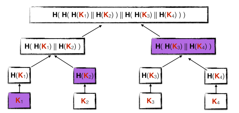
With a hash tree, verifiers of signatures only need to store the root hash of the tree (typically of 256 bits), instead of all the public keys seen as leaves of the tree.

“But the signer needs to store all the private keys, that’s a lot of data!”

Again, there’s a trick, or more precisely a trade-off: instead of storing all the private keys individually, the signer can just store a single secret seed from which the private keys generated (for example, using a pseudorandom function taking as input the index of the key).

Few-times signatures: HORS

Remember that with the Winternitz one-time scheme (WOTS) we were stuck with signing messages of length w, and that increasing the message to useful lengths made signing utterly slow.

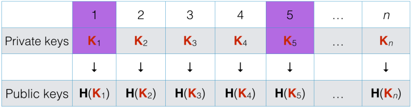
An elegant solution to this problem was provided by Reyzin and Reyzin (father and son) with the Hash to Obtain Random Subset (HORS) construction: given a set of keys K₁ to K_n, a hash function is used to get a few random indices from a given message. The signature is then the private keys with those indices. As showed below, this signing technique is repeated until too many private keys have been released—that is, security degrades with the number of messages signed.

For example, if H(M) = {1, 5}, the signature of M is K₁ and K_5:

Then if you may sign a second message by computing H(M‘) = {2,3}, and releasing K₂ and K₃ as the signature of M‘:

At some point, however, all keys will have been released, and then the scheme becomes useless:

Like WOTS and hash trees, HORS is a key component of the SPHINCS scheme, where a variant called HORST (HORS with Trees) is used in order to reduce the public key size.

Easily finding collisions for any hash

Forget quantum algorithms, if you want to easily find collisions for any hash function, you’ve got to use the biggest quantum computer available: the universe. Right, if you subscribe to the many-world interpretation of quantum mechanics, every possible observation of a quantum phenomena happens in one parallel universe. In particular, if you pick (say) 264 random bits where each of the 264 bits is chosen by observing a distinct quantum state |ψ⟩ = a |0⟩ + b |1⟩, with |a|² = |b|² = 1/2, then each possibility can be seen as happening in a different universe—a different branch of the wave function. You may for example use an off-the-shelf QRNG (although the bits it will spit will have gone through a classical post-processing stage, but that doesn’t matter), or the Universe Splitter application:

Now what?

Concretely, you will first hash the first eight bits with (say) the hash function BLAKE2, read the digest, then hash the last 256 bits, and compare the digest to the first one. If they’re equal, congratulations! You happen to be in one of the few universes where the two messages hash to the same digest. But you’ll have to be very lucky; of the 2²⁶⁴ possibilities, you can expect around 162 collisions. Of the 2²⁶⁴ universes just created, most versions of you will therefore be out of luck.

But if you’ve got a collision, you can not only advertize it and become famous, you can then keep playing: keeping picking random quantum states again and again, and there’ll be a universe where you’re finding a series of collisions one after the other, just by looking!

You may find the idea preposterous, but it’s actually based on serious physics. This model of computer was seriously studied by Scott Aaronson with the concept of anthropic computing, which extends the complexity class BQP (problems that a quantum computer can solve) to the class PostBQP (problems that a quantum computer can solve in parallel universes).

Of course, this kind of cosmological algorithm applies not only to break hash functions but also to recover the secret key of any algorithm, even post-quantum ones. However, informationally secure schemes such as one-time pad encryption will remain safe, since there’s just not enough information out there to determine what’s the correct key—even in parallel universes.