Recently I gave a 4-hour workshop on Timing Attacks at the ZeroNight conference in Moscow. The conference focused on practical software security thus I prepared following “real” Timing Attacks against AES and DES software implementations:
- Trivial DES implementation.
- Trivial AES implementation.
- “Secured” AES implementation.
The source code and tens of millions of plaintext/ciphertext pairs with their corresponding execution time were provided during the workshop.
For each of the implementations, including the “secured” AES, it was possible, using timing attacks, to extract the key.
Below a brief, non-technical introduction to timing attacks, is presented. First I introduce the attack’s concept and context by some abstract examples. Later I demonstrate a successful attack on a trivial DES implementation.
I would like to thank Andrew Mclauchlan for proofreading and editing this post. Also I would like to thank all Security Evaluation Lab team members for their valuable comments.
1. INTRODUCTION
Timing Attack (TA) is a basic Side-Channel Analysis (SCA) method first published at CRYPTO’96 by Paul Kocher. This method allows extraction of an algorithm’s secret, such as a master key, if the algorithm’s execution time depends on a user input and this secret. TAs have mostly been applied in cryptography, however there are other possible attack targets.
The basic attack’s idea is to build time model, i.e. predict execution time, on the basis of a user input and a small part of the secret. For each input and a chosen part of the secret a user models the execution time then he compares the real and modelled execution times. When the guessed part of the secret is correct the timings shall correspond.
Usually, TAs are considered as attacks against badly written code thus TAs are assumed to be useless in ‘professional’ and protected environments. This is not 100% true. First of all, TAs have been successfully applied against OpenSSL code: example 1, example 2. Secondly (and surprisingly) TA methods can be adapted for other ‘protected’ environments, for example to find filenames on WebServers (as demonstrated by Ivan Novikov in his talk Filesystem timing attacks in practice, also at ZeroNights). Thirdly, TAs are evolving and new attacks, which exploit middleware and hardware time differences such as cache hits and misses, are being developed. That is why TAs are still important and, perhaps, may be applied in the field.
2. TIMING ATTACK BASICS
This section demonstrates a simple example of a timing attack. No hard maths nor academic notations are presented here.
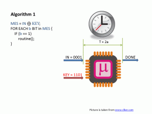
Consider the following extremely simple example shown in Figure 1. Here a microcontroller executes an Algorithm based on a 4-bit value as follows.
MES = IN XOR KEY;     // Exclusive-OR the input with the secret Key
FOR EACH b BIT in MES // For each bit of the resulting value (MES):
{
 IF (b == 1)
   routine();         // Perform a certain calculation only if bit = 1
}
The algorithm performs a bit-wise Exclusive-OR between the user provided input (IN) and the secret key (KEY) and stores it (MES). Each bit of MES is checked. If the bit is one a calculation (routine) is performed, if the bit is zero the calculation is not performed. One routine execution takes 1ms.
Once all bits of MES have been handled the algorithm has finished and reports this to the user. Of course the intermediate value MES is not reported or it would be easy to extract the key.
Click to enlarge

The user knows the algorithm but he does not know the KEY and he really wants to know it. So what does he do?! He measures the execution time for each given input IN as shown in the table below:
| User input, IN | Exec. time |
|---|---|
| 0001 | 2 ms |
| 0010 | 4 ms |
| 0011 | 3 ms |
| 0100 | 2 ms |
Since the user knows Algorithm 1 he also knows that the execution time depends on individual bits of MES; hence, he can predict how much time Algorithm 1 would take for an arbitrary key KEYj and input INi. Trying all possible KEYj values he can find the one that corresponds to the real measurements.
So to get the value of KEY he can:
- take an arbitrary key value KEYj: j in [0:15]
- compute the XOR between the KEYj and all possible values of IN
- calculate the number of bits for each of the XORed values
- compare the predicted number of bits for each key guess to the measured time of the algorithm with unknown key
| User input | Time prediction for KEY0=0000 | Time prediction for KEY1=0001 | Time prediction for KEYj=XXXX | Time prediction for KEY13=1101 | Exec. time |
|---|---|---|---|---|---|
| 0001 | 1 | 0 | … | 2 | 2 ms |
| 0010 | 1 | 2 | … | 4 | 4 ms |
| 0011 | 2 | 1 | … | 3 | 3 ms |
| 0100 | 1 | 2 | … | 2 | 2 ms |
This example is obvious; however, in reality the situation is more complicated: the algorithm might process additional time-variant information, the measurements may not be perfect, there are additional instructions in the code that add noise, etc. Intuition says that in the real case a timing attack would not be possible. Intuition is wrong.
In order to explain why intuition is wrong I present an extended example in the following chapter.
3. EXTENDED EXAMPLE
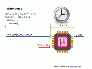
Consider the same microcontroller and the same algorithm as before with only some small differences: the user knows (and controls) only four bits of the message out of a 128-bit message. The 128-bit key consists of four bits repeated thirty two times.
As before the input message IN is XORed with the secret KEY and the result is stored in the variable MES. Now MES is 128-bits long so the user can not measure directly the time to treat the four bits which he directly controls, but instead will measure the time to process all of the bits of MES.
Click to enlarge

The user does not know the additional 124 input bits, but assumes that they are randomly changing. As before he records the time for each given four bits input that he controls. The execution time in this case would become the form of: INi and corresponding measured time Ti as shown in the table below:
| User input INi | First measurement | Second measurement | Nth measurement |
|---|---|---|---|
| 0001 | 64 ms | 58 ms | 72 ms |
| 0010 | 57 ms | 79 ms | 83 ms |
| 0011 | 89 ms | 59 ms | 64 ms |
| 0100 | 49 ms | 78 ms | 67 ms |
It is important to note that as the 124 unknown input bits may be randomly changing, the user will measure different execution times for the same four bit input.
What would a user do in this case? To answer this question I would like firstly to introduce (or remind) Law of large numbers. According to this law “the average of the results obtained from a large number of trials should be close to the expected value, and will tend to become closer as more trials are performed”. I call the Law of large number the side-channel attacker’s best friend.
What does this law practically mean for timing attacks?! Well, if a user performs a lot of executions of an algorithm with the same 4bit input and then averages the execution time for all of them the random part (i.e. the time introduced to process the 124 bits outside the user’s control) will tend towards a constant value. To demonstrate this I wrote a small code in Matlab which performs the above algorithm for a fixed key with the user controlling four bits and the remaining 124 bits changing randomly:
function LawBig()
colors = ['r','b','k','g'];

%precomputed hamming weights for all 0:255 values
HWTab  = sum( dec2bin(0:15).' == '1' );

%The KEY
key = 3;

N = 3000;
sumBits = zeros(16,N);

figure;
hold on;
for iCtrlIN = 0:15
 for iCnt = 1:(N-1)
 %Simulate random number of bits in the MES
 unknownMesBits = round(rand(1,124));

 %Compute the controllable part of the MES
 knownMes = bitxor(uint8(iCtrlIN),uint8(key));

 %Compute the number of bits in the entire MES
 allMesBits = HWTab(knownMes + 1) + sum(unknownMesBits);

 %Add the number of bits
 sumBits(iCtrlIN+1,iCnt+1) = sumBits(iCtrlIN+1,iCnt)+ allMesBits;
 end
 plot(1:N,sumBits(iCtrlIN+1,:) ./ (1:N),colors(mod(iCtrlIN + sum(unknownMesBits),4)+1));
end
hold off;

xlabel('N of executions','FontSize',24);
ylabel('Average number of bits (or average time)','FontSize',24);
set(gca,'FontSize',24);
end
According to the Law of big numbers after several executions the average contribution to the execution time by the unknown, randomly varying, part will converge on the mean value.
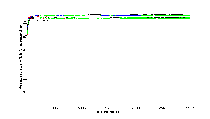
The output of the Matlab simulation is shown in Figure 3 (clickable), with a zoom in Figure 4 (clickable) this confirms that this example conforms to the law of bit numbers.
Click to enlarge

Figure 3 demonstrates how the average execution time quickly converges towards the mean value only after a few hundred executions. In Figure 4, after 3000 executions, the mean value has been reached. It can be seen that the shortest execution time corresponds to the “routine()” being executed 0 times (for the known 4 input bits) and that the other curves converge around values which can be expressed as a constant (the shortest time) plus a multiple of a certain time. Using this information the attacker can construct a table similar to that of the initial example.
Click to enlarge

| User input | Averaged time |
|---|---|
| 0000 | 2 + const |
| 0100 | 3 + const |
| 0111 | 1 + const |
| 1100 | 4 + const |
Now trying all possible KEY values (4 bits) the user can build a time prediction and compare the real time and the modelled time as it was done before.
Comparing this manually is not much fun. To automate the comparison side-channel attacks use statistical tools known as distinguishers. These statistical tools show if dependency exists between two variables. For this concrete example we can apply the Pearson Correlation Coefficient (PCC), but there are also Mutual Information, Kolmogorov-Smirnov among others. PCC shows if there is any linear dependency between two variables, i.e. should two variables x and y have a relationship y = ax + b (a,b are constants), then PCC will give a result equal to 1, otherwise PCC will give a much smaller value (e.g. as shown in WikiFigure1 and WikiFigure2).
To conclude the two previous sections:
1. Law of big numbers is the side-channel attacker’s best friend, because it averages all noise sources to a constant value.
2. Distinguishers (like Pearson Correlation Coefficient) are also of a great aid for Side Channel Attack as they help to identify if a model is close to the real implementation.
Now I would like to present the ‘real’ case example against DES algorithm.
4. DES C++ STRAIGHTFORWARD IMPLEMENTATION
In this simple example we consider the P-permutation of the DES algorithm implemented in the following way:
uint32_t DES_P(const uint32_t input)
{
/*This function permutes 32-bit input*/
int iBit = 0;
uint32_t res = 0x0ULL;
uint32_t one = 0x1ULL;

/*VULNERABLE TIME-VARIANT OPERATION*/
for (iBit = 0; iBit < 32; iBit++)
 if ( GET_BIT(input,32 - p_table[iBit]) == 1 )
  res |= one << (31 - iBit);
return res;
}
Compiled for x86 processor (iCore7, 8GB RAM, Linux Mint 14) with g++ option -O2 (optimization option 2), the following assembler code was created:
...
xorl %eax, %eax          //Make the register equal to 0
...
movl $31, %edi           //Store the value 31 in %edi
...
movl 20(%esp), %esi      //Store the value from stack to the %esi (apparently this is input)
movl $32, %ebx           //Store the value 32 in %ebx
...
.L22:
movl %ebx, %ecx          //Store 32 in %ecx
subb p_table(%edx), %cl  //Value p_table(%edx) = p_table(iBit) is subtracted from 8 least significant bits of the counter register (%cl). The result is stored in those 8 bits, i.e. 32 - p_table[iBit]
btl %ecx, %esi           //Bit of %esi (input) shifted by (32 - p_table[iBit] = %ecx) is set to the carry flag, i.e. GET_BIT(input,32 - p_table[iBit])==1
jnc .L21                 //Jump if not carry, i.e. if the previously stored bit is 0
movl %edi, %ecx          //Move %edi to %ecx, i.e. move 31 to %ecx
movl $1, %ebp            //Move 1 to %ebp
subl %edx, %ecx          //Substruct %edx from %ecx and store the result in %ecx, i.e. 31-iBit
sall %cl, %ebp           //Shift the register %ebp (1) by 8 leas significant bits of %ecx and store the result in %ebp, i.e. 1 << 31-iBit
orl %ebp, %eax           //Compute OR between the initially empty register (%eax) and the %ebp (1 << 31-iBit), keep the result at %eax
.L21:
addl $1, %edx            //Increase the loop counter (iBit++)
cmpl $32, %edx           //Set the carry flag to 1 if counter == 32, i.e. iBit<32
jne .L22 //If counter is still less than 32 continue the loop
Lines 14 to 18 of the assembler code (corresponding to lines 10 to 11 of the C code) are executed only if the instruction in line 12 set the carrier bit to 1, i.e. a certain calculation is only performed for certain conditions based on the value of some input bits. This is similar to the example provided in Algorithm 1. Thus this DES implementation is vulnerable!!!
Consider that a user can control the DES input plaintext can also measure the total DES execution time. In this case he can perform a lot of encryptions and store plaintext/ciphertext pair with corresponding execution time.
How the actual attack is performed?! Consider only the first round of DES on Figure 5 (clickable).
Click to enlarge

Here, R, a subset of the plaintext input is expanded by E, XOR’d with the unknown Subkey then the resulting 6-bit value is used to output a 4-bit value from the substitution box (Sbox).
We know the plaintext, so we can easily compute R. All the internal operations, i.e. E expansion, Sbox output values and P permutations are known. The only unknown part is the Sub key. As highlighted above the execution time depends on the number of input bits to the block P (see the C code). In fact, we can compute IN2P the input to the P permutation (see the Figure 5):
IN2P = Sbox[E(R) ⊕ SubKey] (1)
Since each Sbox is independent we can write this expression only for the first 4 bits:
IN2P1..4 = Sbox1[E(R)1..6 ⊕ SubKey1..6] (2)
Now we need to compute the number of bits in the variable IN2P1..4 and this is going to be our time model. The number of bits in IN2P1..4 is denoted by HW(IN2P1..4) – Hamming weight of IN2P1..4. That is it, we have just created the time model for the 4 input bits of first P permutation (3):
HW(IN2P1..4)= HW(Sbox1[E(R)1..6 ⊕ SubKey1..6]) (3)
In the above expression (3) we know everything except the bits of SubKey. Next we compute the expression (3) for each SubKey value and all available plaintexts (50 millions available during the workshop). This lead to 64 time models for each Subkey value.
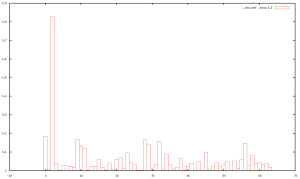
Following to the previous explanations those 64 models must be correlated with the real execution time. Figure 6 shows the result using 50 million plaintexts. Here the X-axis is the Subkey value and Y-axis is a value of the pearson correlation coefficient (PCC) multiplied by some constant.
It can be seen that the correlation for the Subkey value 2 is by far the largest and indeed this value is correct.
Click to enlarge

As usual intuition says that the above demonstration should not work because of a variety of reasons: we compute only 4 bits of one round and there are 16 rounds in DES, each round has 32 bit input into the P permutation, timing measurements are not perfect, the DES calculation done by PC is too quick, etc. However, do you remember the Side Channel Attack’s best friend? The law of big numbers!
All of the noisy parts shall be averaged after certain number of encryptions. It may be 10,000,000 encryptions or 40,000,000 (we don’t know in advance), but at the end all the noise will be averaged to a constant. So by trying all possible 6 bits of the first SubKey input to the Sbox1 we can find the correct SubKey value.
To find the entire first round key we can compute time models for all Sbox outputs. One can apply similar attack on the last DES round P permutation. In fact there are a lot of attack’s advancments that can decrease the number of required encryptions: make a time model for two Sbox outputs, take into account the first and last DES rounds, perform an attack on the second round when the part of the first Subkey is recovered, etc.
Anyway, the goal of this tutorial was to introduce Timing Attacks to a non-technical person. I was trying to highlight three main points:
- When any physical parameter (time in this workshop) depends on the fixed secret and variable known data, the secret can be extracted by Side Channel Attacks.
- Noise is not a big issue for Side Channel Attacks because as stated by the Law of big numbers any noise can be averaged.
- Distinguishers help to choose the correct key candidate as they show wheather a modelled and a real data are linked.
For the moment that is all I wanted to say. If you have any questions for the timing analysis description, don’t hesitate to ask them in the comments. The second part of this tutorial will follow soon. It will include an attack on vulnerable and ‘protected’ AES software implementations.
If you would like to complete the workshop yourself you can find the source code here. The archive includes two folders. The folder ‘src’ has all the source files used in the workshop. The folder ‘bin’ has a Makefile and the binaries used in the project.
The sources can be compiled by g++ and omp library (included automatically to g++). You may compile this code under both Linux and MacOs (some people also used Cygwin to compile the code during the workshop).
To compile the project use terminal and type make in the ‘bin’ directory. To generate the required timing data for the DES implementation I have also supplied a function:
CreateTimeDatabase(nEnc, realtimeFilename, plaintextFilename);
that will execute nEnc encryptions and store all plaintext in plaintextFilename file and the corresponding execution time in realtimeFilename file. Chose a sufficiently large value for nEnc (around 50 millions).
Then you can try to analyse the generated data with the following function:
TimingAttackDES_OneSbox(nEnc, realtimeFilename, plaintextFilename, resultFilename, byteToRecover);
where byteToRecover is the number of Sbox which output will be used for attack; resultFilename is the file that keeps pearson correlation coefficients for each SubKey value.
Once TimingAttackDES_OneSbox is finished you can plot the resultFilename using gnuplot (or any other tool).


2 comments